

Research on the application of the Quantum-behaved Particle Swarm Optimization algorithm in the inverse estimation of in-situ stress based on fault-slip fractures
-
摘要: 为了提高断层滑动数据中应力张量反演的计算效率与精度,解决传统网格搜索方法计算耗时大、易陷入局部最优等问题,开展了基于智能优化算法的应力反演研究。文章提出了一种基于Quantum-behaved Particle Swarm Optimization(QPSO,量子群优化)算法的断层滑动数据反演方法,将应力张量参数化为应力主轴方向的3个欧拉角(α、β、γ)及应力比(Φ)构成四维变量,构建以剪切力−滑移夹角为核心的适配度函数;通过借鉴精英学习策略,引入奖惩反馈机制和张量距离量化方法以提高个体搜索能力与种群多样性。利用模拟断层数据集,设定多组应力模型,通过对比网格搜索法与QPSO反演法的识别效率与精度,开展反演效果验证。结果表明,所提出的QPSO反演法在非收敛率低于8%条件下,反演时间仅为传统方法的约1/27;在高维多峰复杂空间中亦可快速收敛,准确识别出正断型、逆断型与走滑型应力状态,聚类效果清晰,表现出良好的稳定性和物理一致性。该方法在断层滑动信息反演地应力场方面具有显著优势,具备计算效率高、适应性强、收敛速度快等特点,可为区域地应力场反演、震源机制分析等提供有效技术支撑,并为智能优化算法在地质力学领域的深度融合提供了理论方法的启示和借鉴作用。Abstract:
Objective To improve the computational efficiency and accuracy of stress tensor inversion from fault-slip data, and to address the limitations of conventional grid search methods—namely, high computational cost and susceptibility to local optima—an inversion approach based on intelligent optimization algorithms was investigated. Methods A novel fault-slip data inversion method based on the Quantum-behaved Particle Swarm Optimization (QPSO) algorithm is proposed, in which the stress tensor is parameterized by four variables: three Euler angles (α, β, γ) representing the orientations of the principal stress axes and a stress ratio (Φ). A misfit function is constructed based on the angular deviation between the shear stress direction and the observed slip vector. To enhance convergence performance, an elite-guided learning strategy was adopted, incorporating a reward-penalty feedback mechanism and a tensor distance metric to quantify stress similarity. Multiple synthetic stress models were tested using a simulated fault-slip dataset, and the inversion performance of QPSO was compared with the conventional grid search method in terms of efficiency and accuracy. Results The proposed QPSO-based inversion method achieves a non-convergence rate below 8% and reduces computational time to approximately 1/27 of what is required by the grid search approach. The method converges rapidly in high-dimensional, multimodal parameter spaces and accurately identifies normal, reverse, and strike-slip stress regimes. The well-defined clustering of the inversion results indicates strong stability and physical consistency. Conclusion The QPSO-based method exhibits significant advantages in stress tensor inversion from fault-slip data, including high computational efficiency, strong adaptability, and fast convergence. Significance It provides effective technical support for regional in-situ stress field reconstruction and focal mechanism analysis, and offers the enlightenment and reference value of theoretical methods in geomechanical applications. -
Key words:
- stress tensor inversion /
- fault-slip data /
- in-situ stress /
- QPSO inversion method /
- tensor distance
-
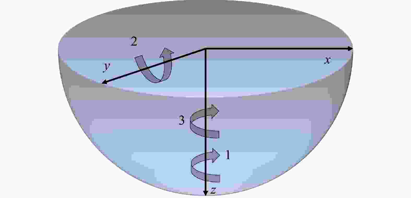
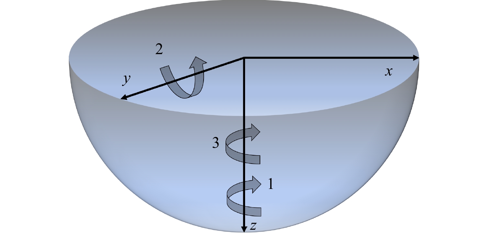
图 2 欧拉转动示意图
图中数字代表转动顺序
Figure 2. Schematic diagram of Euler rotation (digits represent the order of rotation)
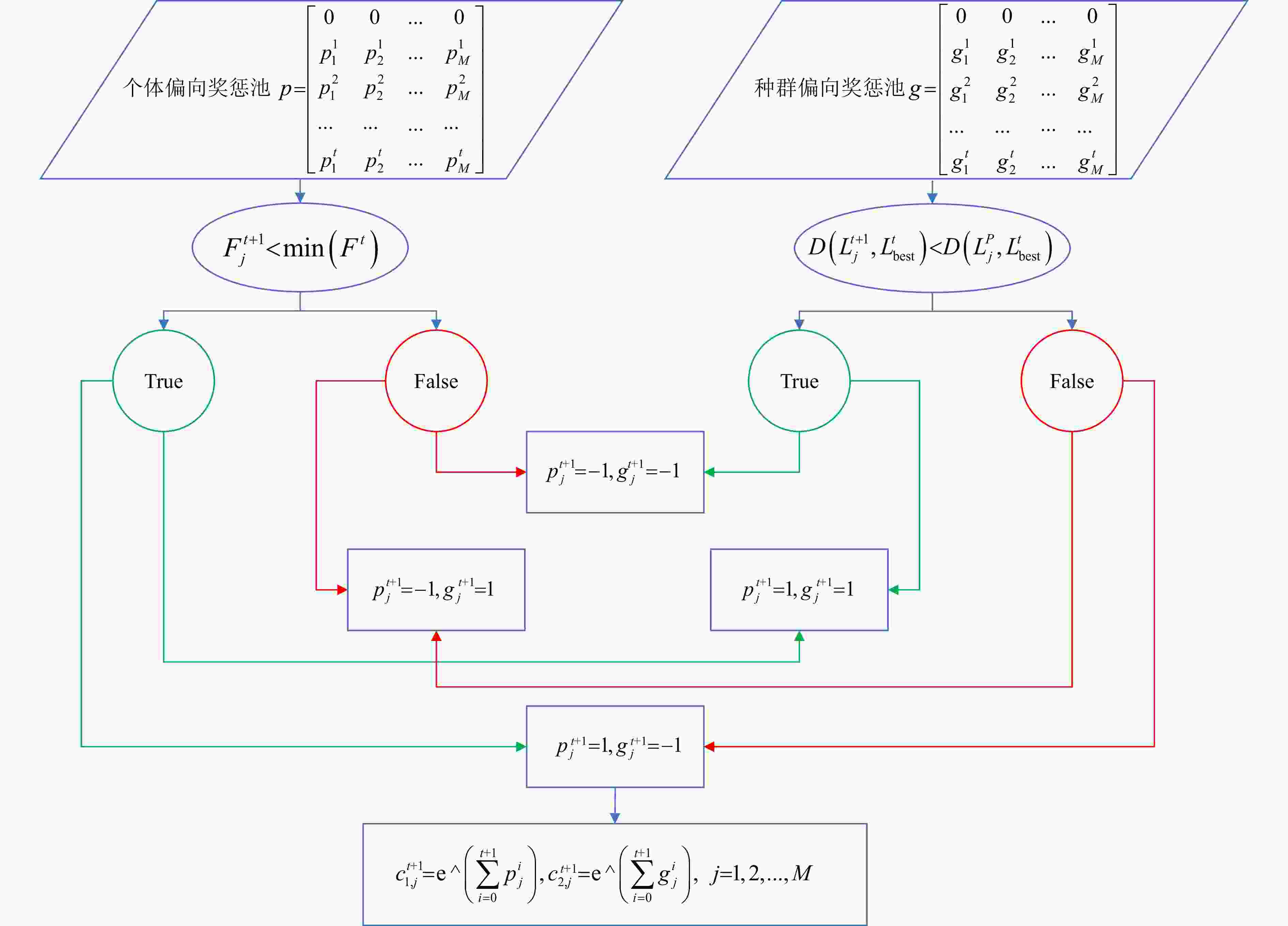
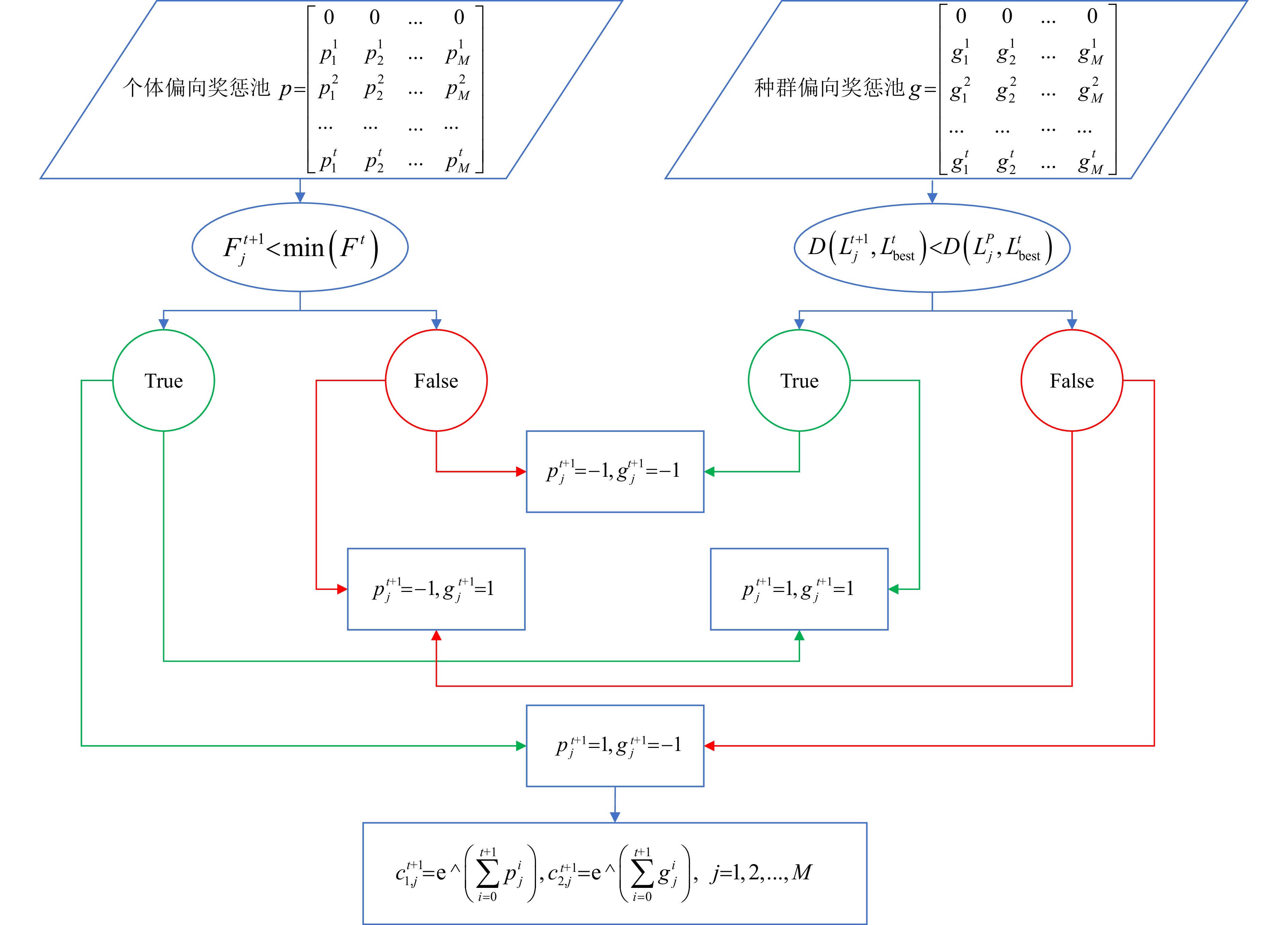
图 3 第t+1次迭代中偏向学习系数的计算流程
t—种群迭代次数;M—种群个体总数;p—个体偏向奖惩池;$ {}_{}^{} $pij—种群中第j个量子在第i次迭代中的个体偏向学习系数;g—种群偏向奖惩池;$ {}_{}^{} $$ {}_{}^{} $$ {}_{}^{} $$ {}_{}^{} $gij—种群中第j个量子在第i次迭代中的种群偏向学习系数;$ {{{F}^{{t}}}\mathrm{\mathrm{\mathrm{ }}}}\text{=}\left[{{F}_{\text{1}}^{{t}}}\text{,}{F}_{\text{2}}^{{t}}\text{, … ,}{F}_{{M}}^{{t}}\right] $—第t代种群适配值;$ {{F}}_{{j}}^{{t+1}} $—第t+1代种群中量子j的适配值;$ {{L}}_{\text{best}}^{{t}} $—第t代种群中具有最好位置的量子的应力参数;$ {{L}}_{{j}}^{{t+1}} $—第t代种群中量子j的应力参数;$ {{L}}_{{j}}^{{P}} $—种群中量子j经历过的最好位置应力参数;D—张量之间的张量距离;$ {}_{}^{} $$ {c}_{{1, j}}^{{t+1}} $—第t+1代中量子j的个体偏向学习系数;$ {{c}}_{{2, j}}^{{t+1}} $—第t+1代中量子j的种群偏向学习系数;e—自然常数
Figure 3. The calculation process of the bias learning coefficient in the (t + 1)th iteration
t—Population iteration count; M—Total number of individuals in the population; p—Individual bias reward–penalty pool; pij$ {}_{}^{} $—Individual bias learning coefficient of the jth quantum in the ith iteration of the population; g—Population bias reward-penalty pool; $ {}_{}^{} $gij—Population bias learning coefficient of the jth quantum in the ith iteration of the population; $$ F^t\mathrm{\mathrm{\mathrm{ }}}\text{=}\left[F_{\text{1}}^t\text{,}F_{\text{2}}^t\text{, … ,}F_M^t\right] $—Fitness values of the population at the tth generation; $ {}_{}^{} $$ {}_{}^{} $$ F_j^{t+1} $—Fitness value of quantum j in the population at the (t+1)th generation; $ L_{\text{best}}^t $$ {}_{}^{} $—Stress parameter of the quantum with the best position in the population at the tth generation; $ {}_{}^{} $$ L_j^{t+1} $—Stress parameter of quantum j in the population at the (t+1)th generation; $ _{ }^{ }L_j^P $—Stress parameter at the best historical position experienced by quantum j in the population; D—Tensor distance between tensors; $ {}_{}^{} $$ c_{1,j}^{t+1} $—Individual bias learning coefficient of quantum j in the (t+1)th generation; $ {}_{}^{} $$ c_{2,j}^{t+1} $—Population bias learning coefficient of quantum j in the (t+1)th generation; e— Euler’s number.
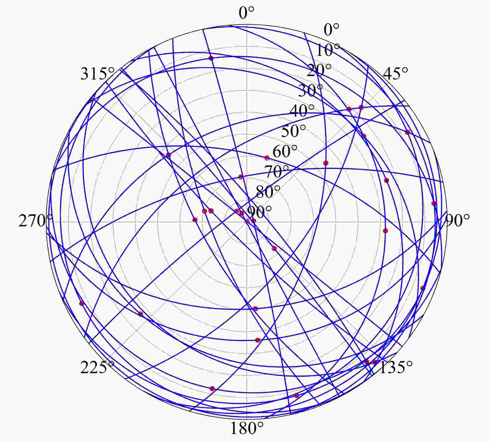
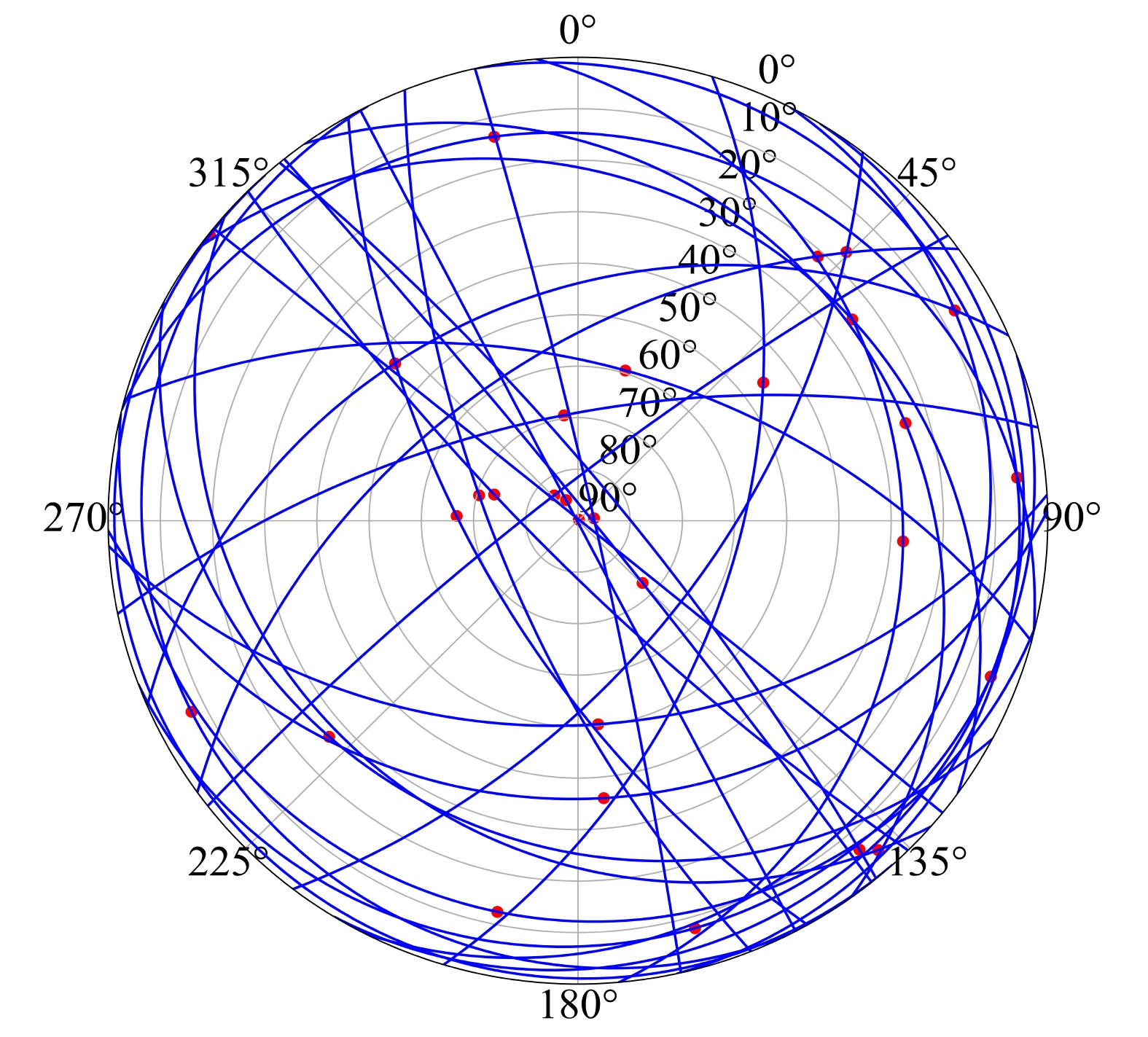
图 4 反演所用断层及滑动方向的下半球投影图
蓝色线为断层投影,红色点为断面滑移方向
Figure 4. The lower hemisphere projection of the faults and slip directions used in the inversion (Note: The blue lines represent the fault projections, and the red dots indicate the slip directions on the fault planes)
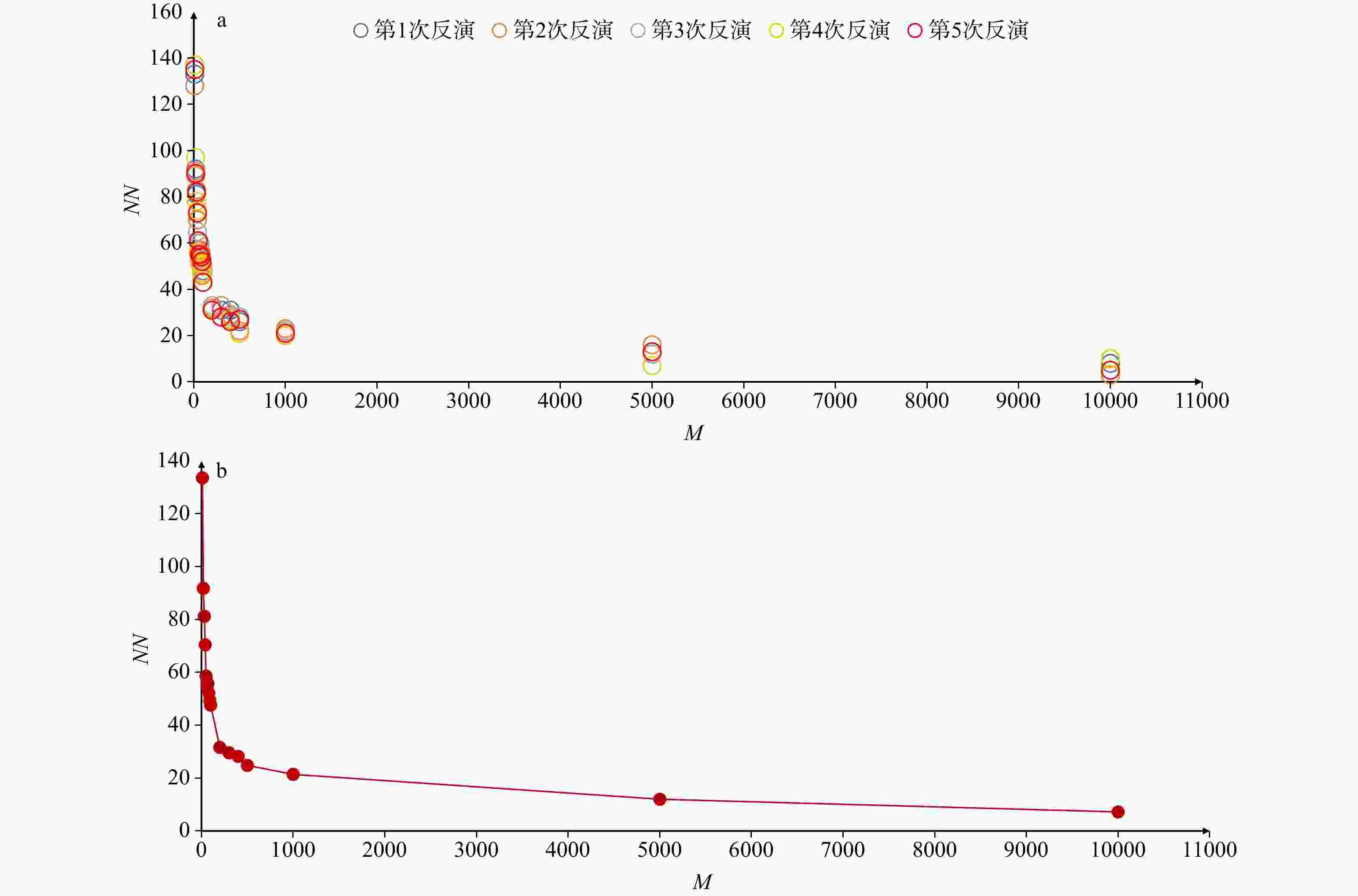
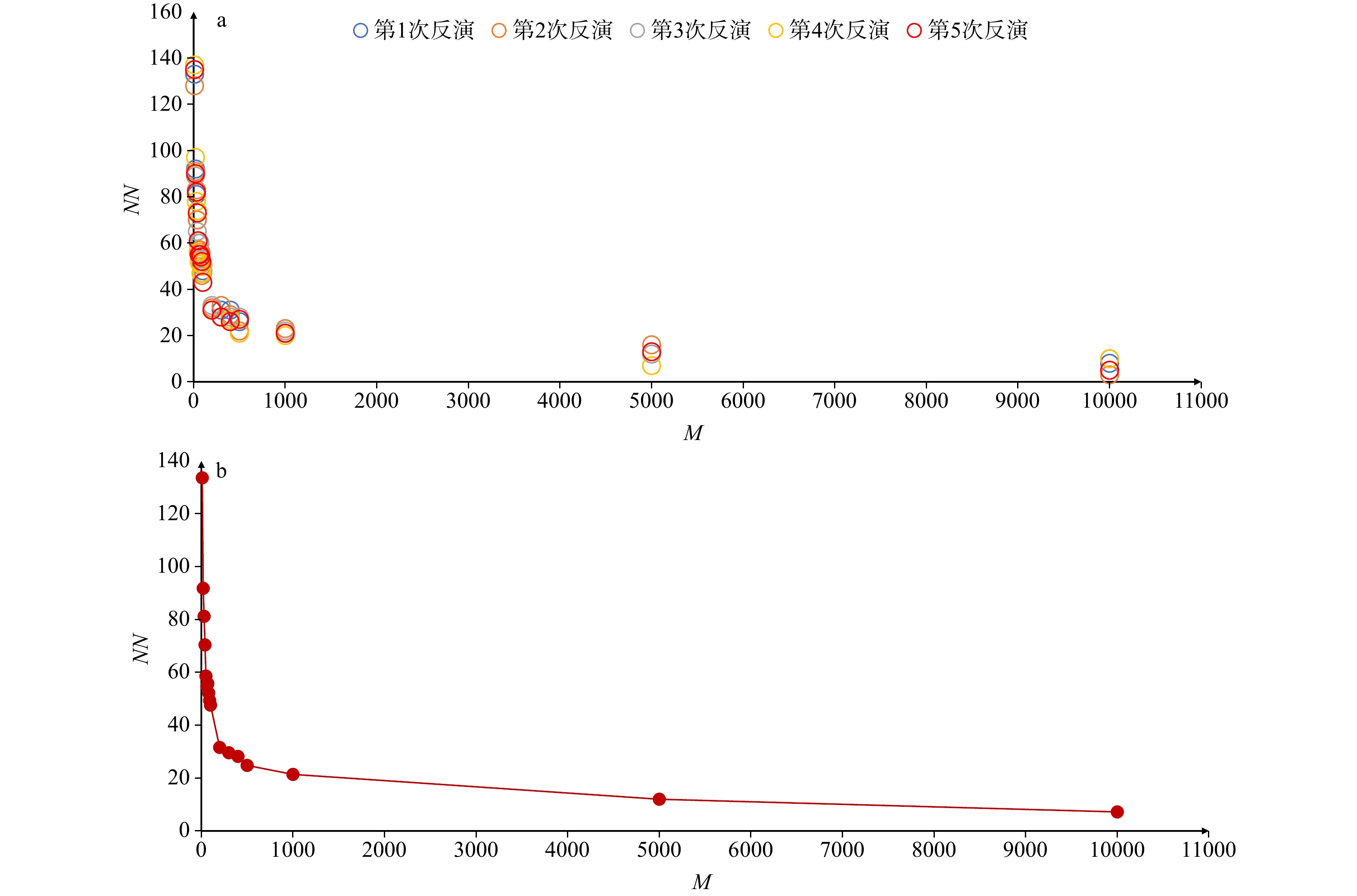
图 5 种群规模M与无法收敛断层组合数量NN函数关系
a—全部反演结果散点图;b—平均值折线图
Figure 5. The functional relationship between population size (M) and the number of non-convergent faults combinations (NN)
(a) Scatter plot of all inversion results; (b) Line chart of average values
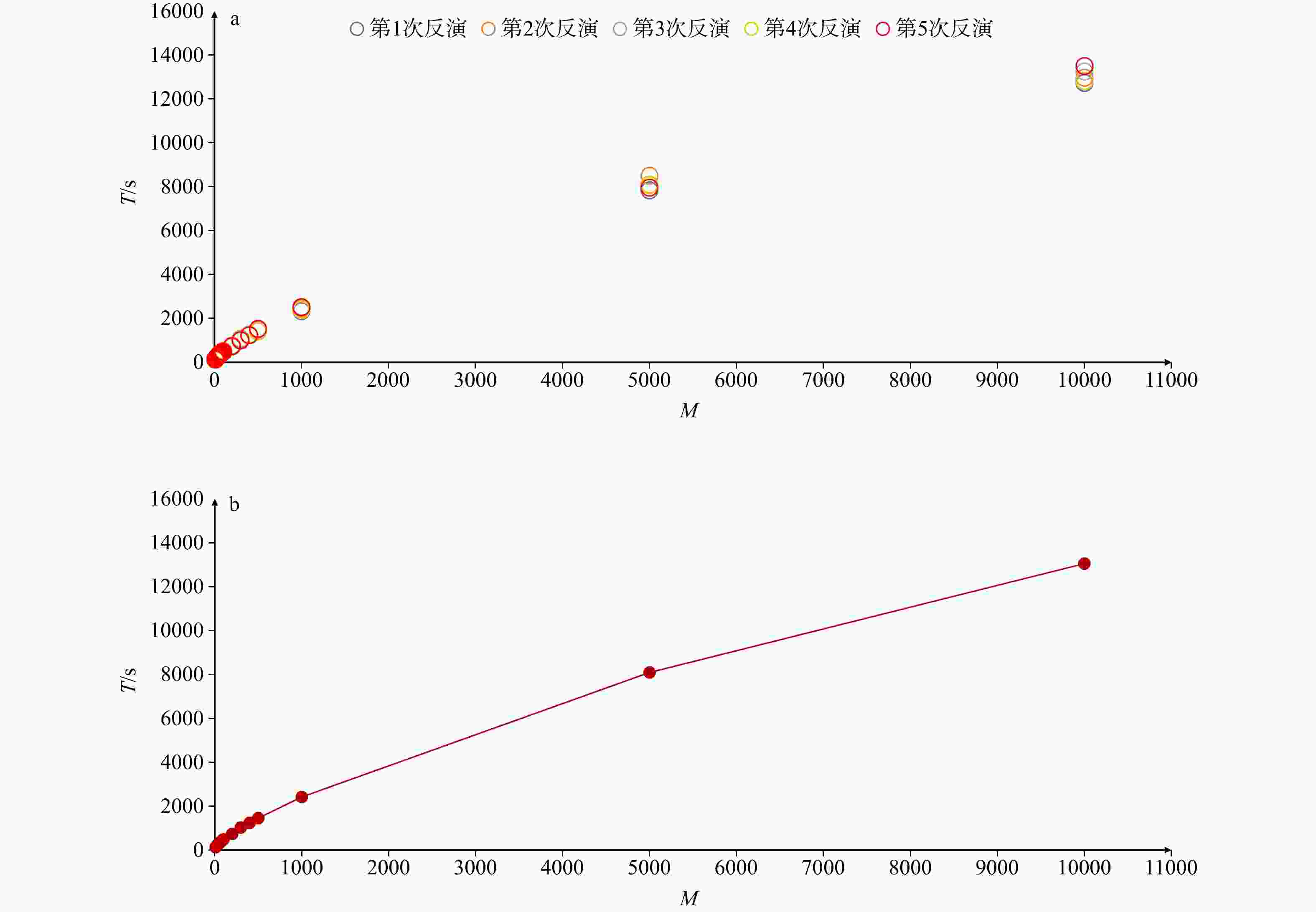
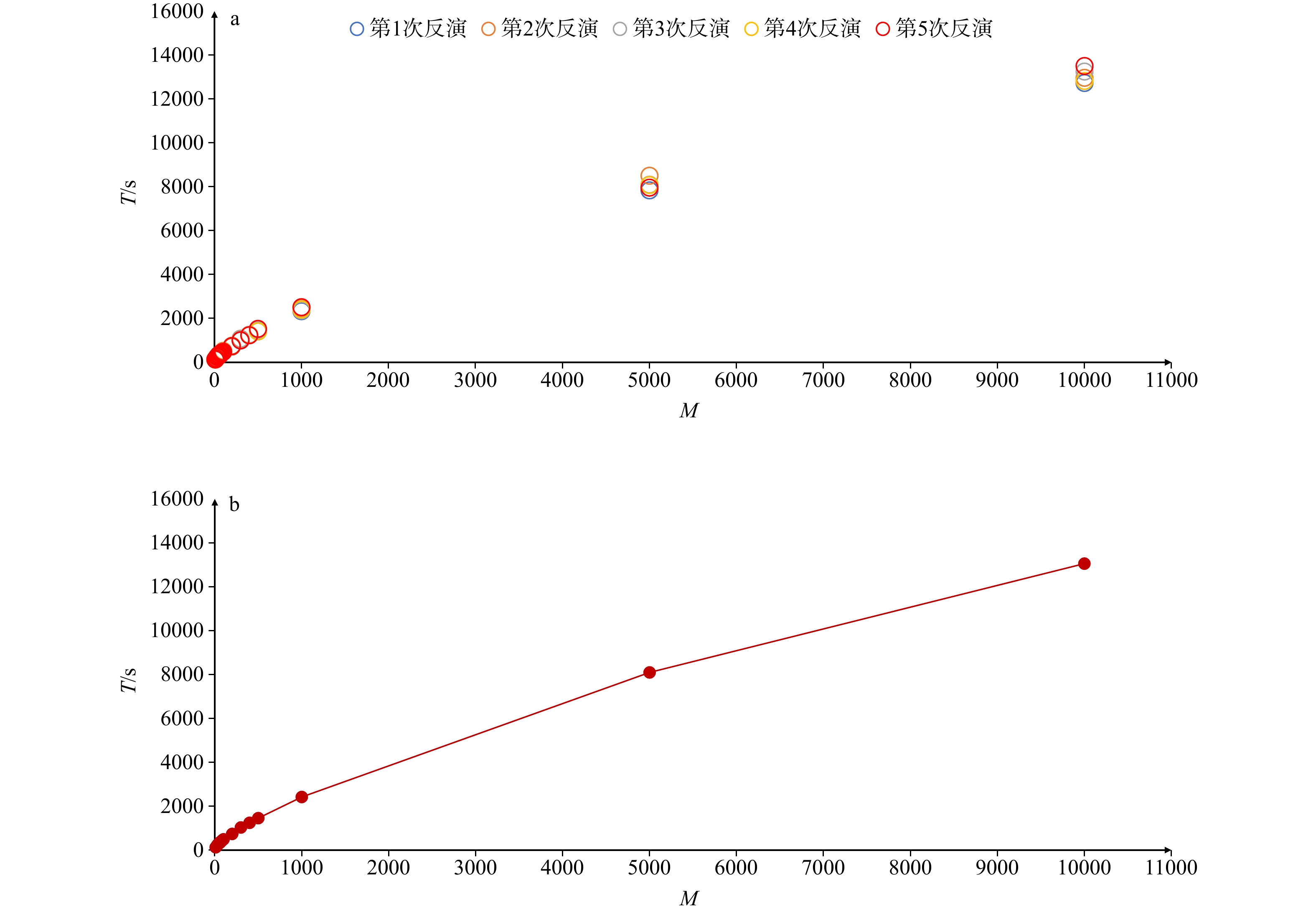
图 6 种群规模M与反演总时间T函数关系
a—全部反演结果散点图;b—平均值折线图
Figure 6. The functional relationship between the population size (M) and the total time of inversion (T)
(a) Scatter plot of all inversion results; (b) Line chart of average values
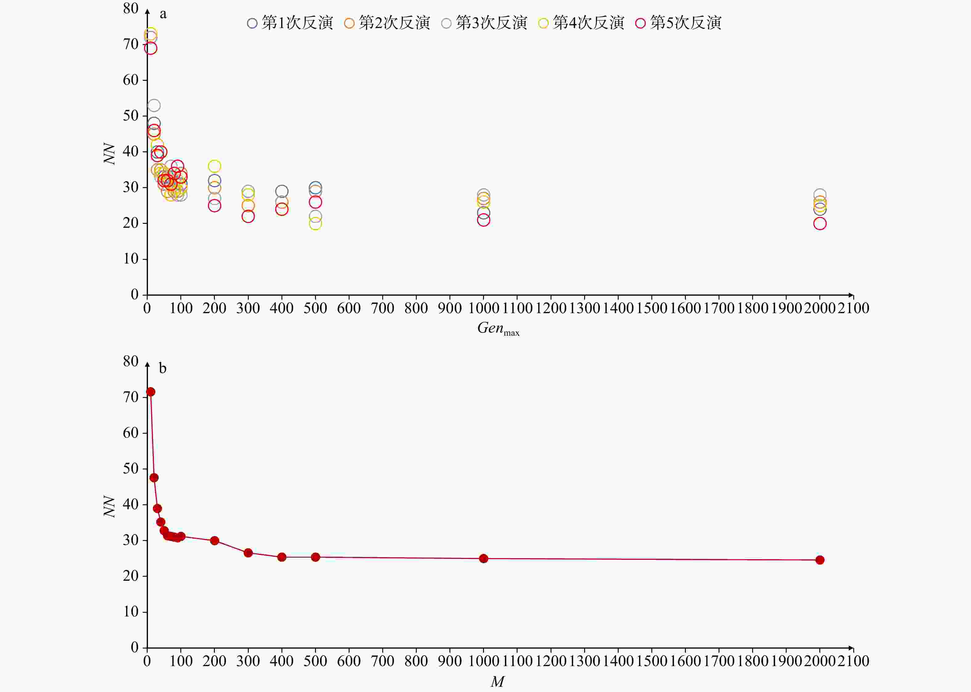
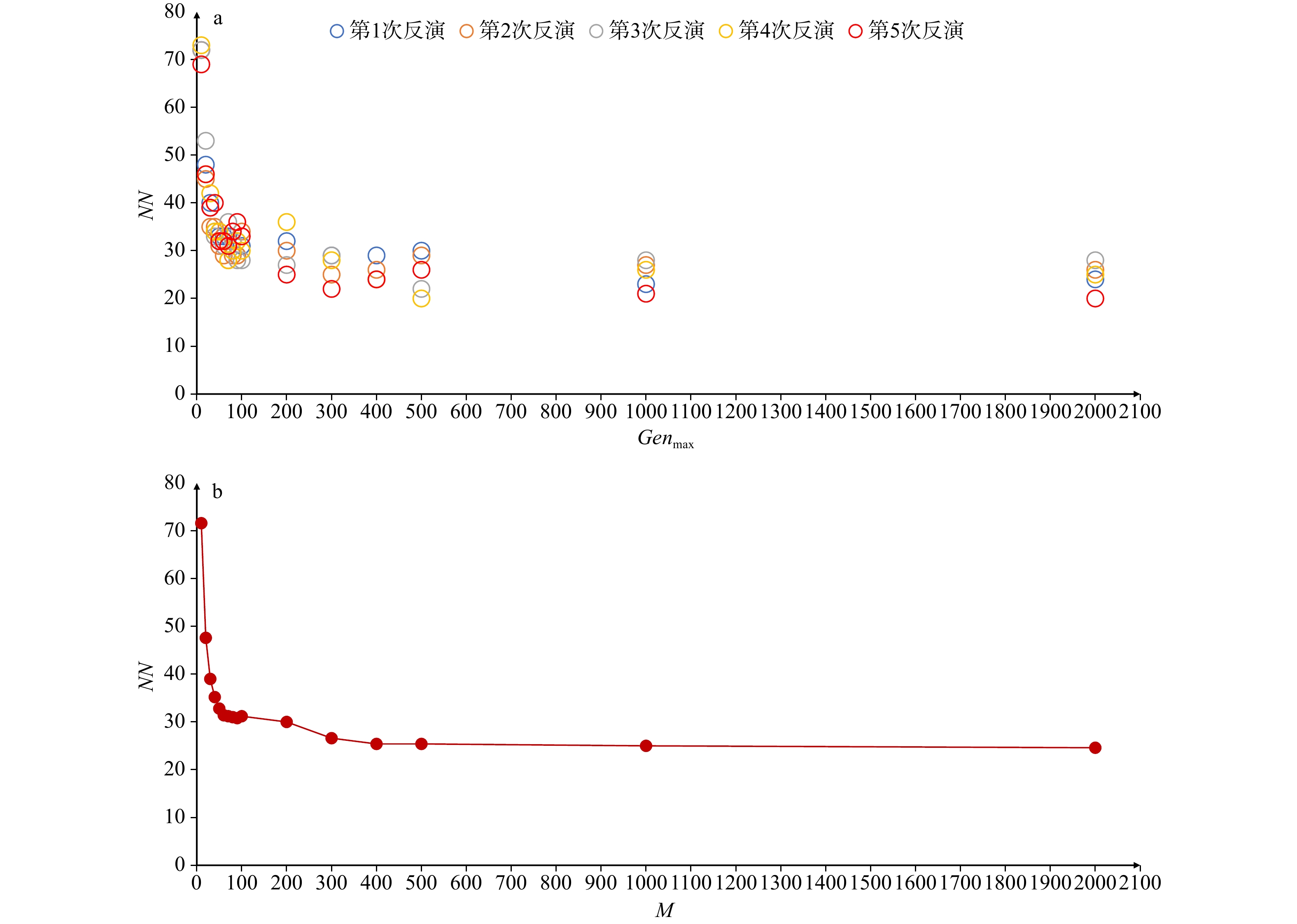
图 7 最大迭代次数Genmax与无法收敛断层组合数量NN函数关系
a—全部反演结果散点图;b—平均值折线图
Figure 7. The functional relationship between the maximum number of iterations (Genmax) and the number of non-convergent fault combinations (NN)
(a) Scatter plot of all inversion results; (b) Line chart of average values
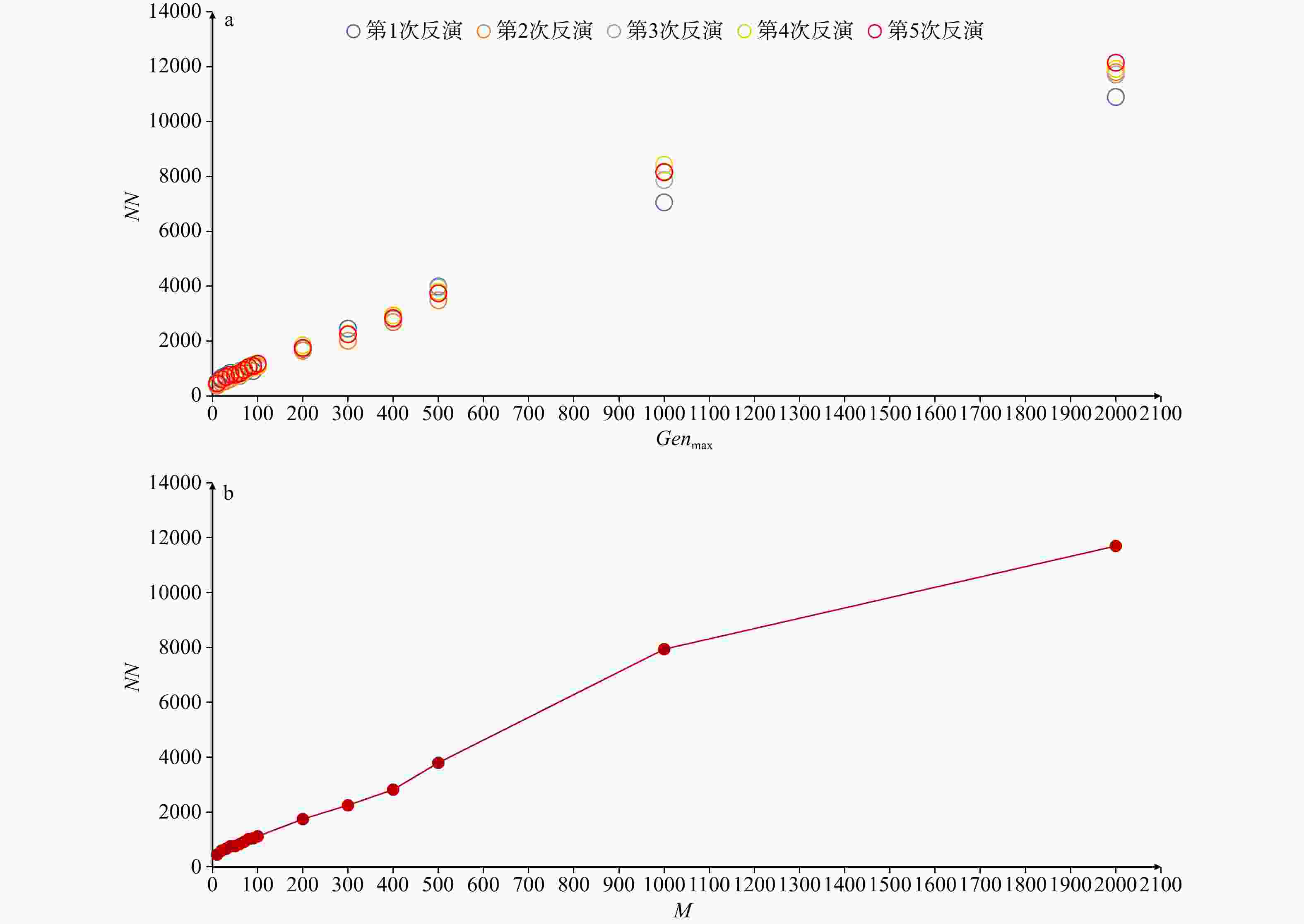
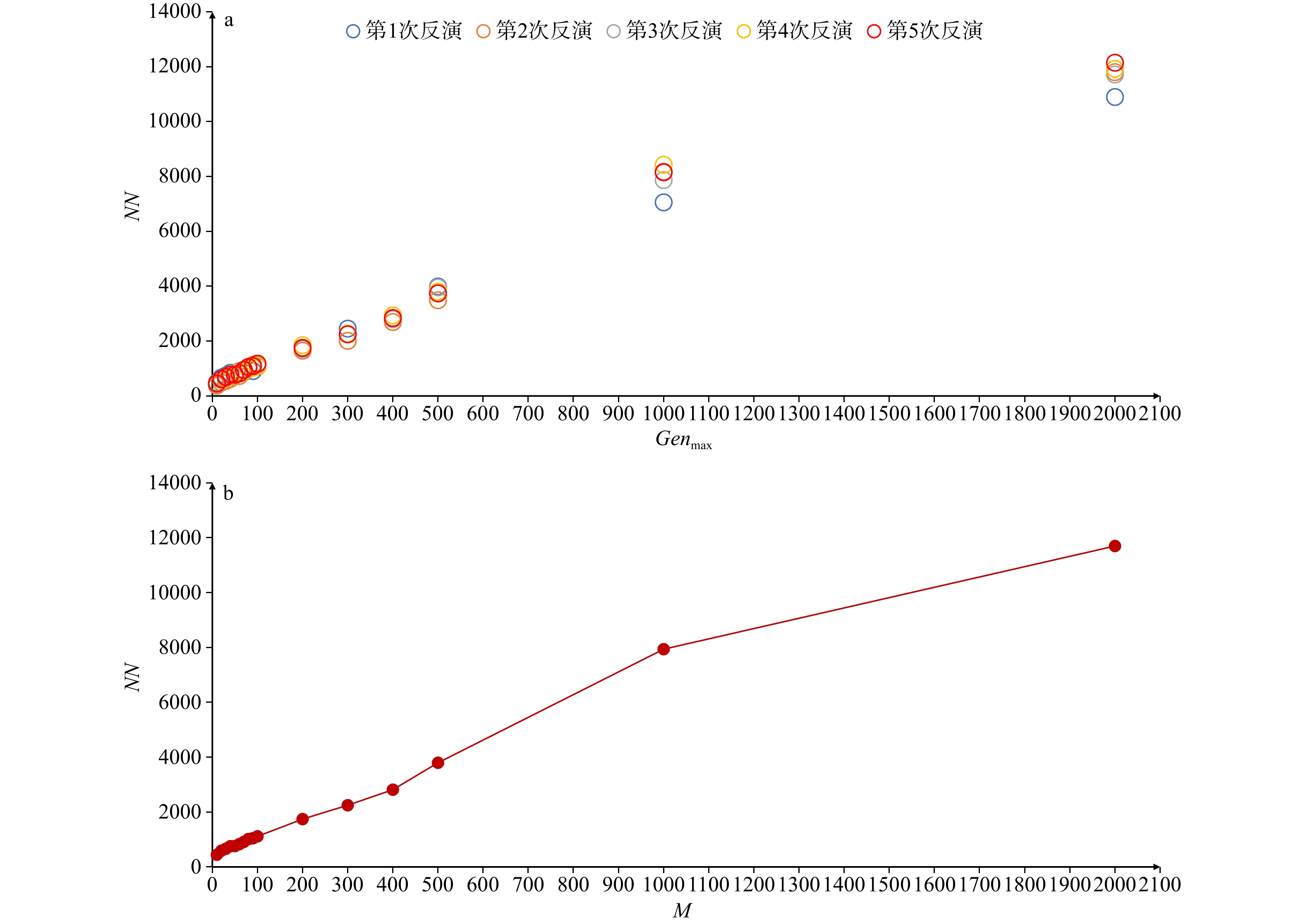
图 8 最大迭代次数Genmax与反演总时间T函数关系图
a—全部反演结果散点图;b—平均值折线图
Figure 8. The functional relationship between the maximum number of iterations (Genmax) and the total time of inversion (T)
(a) Scatter plot of all inversion results; (b) Line chart of average values
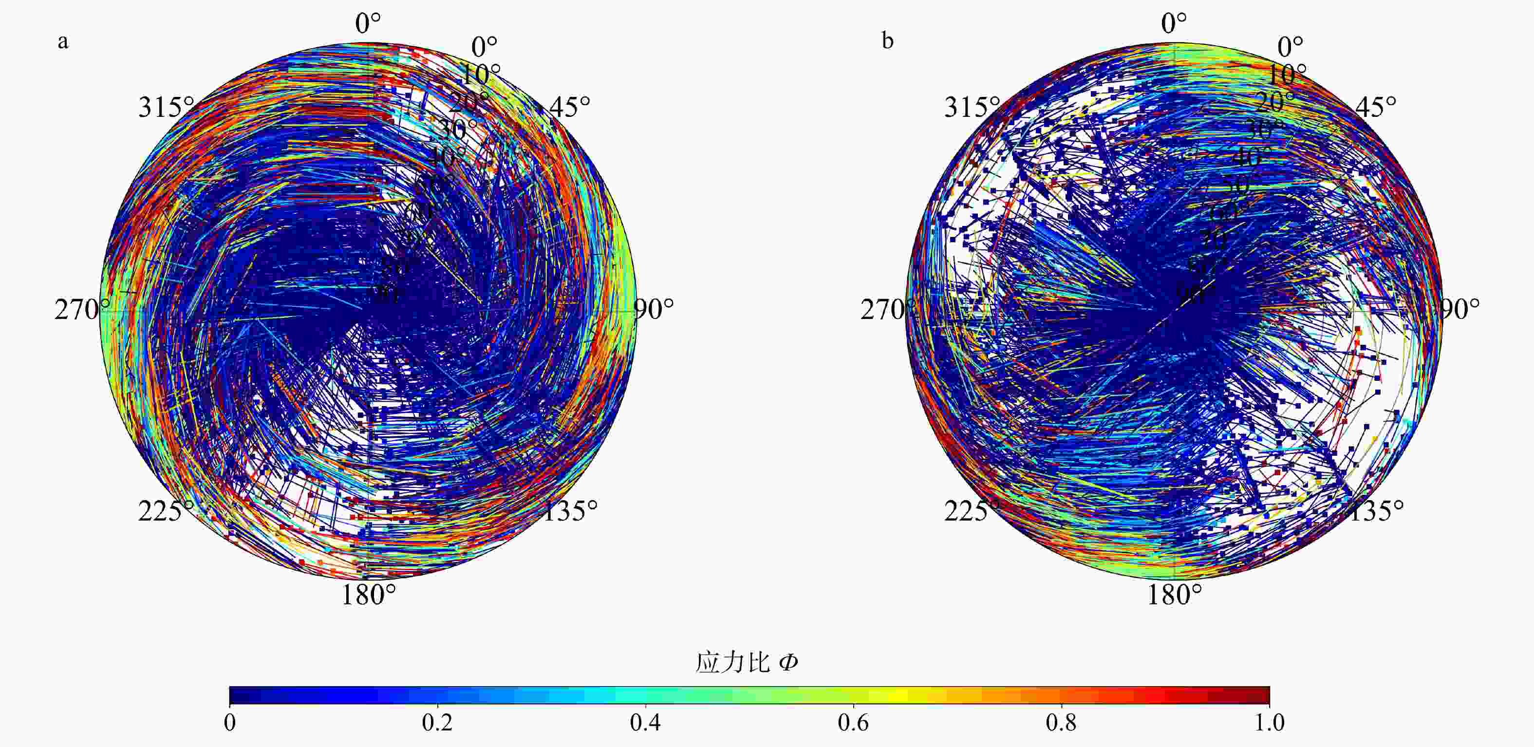
图 9 全部应力结果可视化图像
a—以下半球上的投影点表示σ1轴方向的应力可视化图像(σ3轴的方向用点上的线条表示,分别用线条的方向和长度表示σ3的方位角和倾角);b—以下半球上的投影点表示σ3轴方向的应力可视化图像(σ1轴的方向用点上的线条表示,分别用线条的方向和长度表示σ1的方位角和倾角)
Figure 9. Visualization of total stress results
(a) The projected points on the lower hemisphere visualize stress in the direction of the σ1-axis (The direction of the σ3-axis is indicated by lines attached to the points, and the orientations and lengths of the lines represent the azimuth and dip angle of σ3, respectively.); (b) The projected points on the lower hemisphere visualize stress in the direction of the σ3-axis (The direction of the σ1-axis is indicated by lines attached to the points, and the orientations and lengths of the lines represent the azimuth and dip angle of σ1, respectively.)
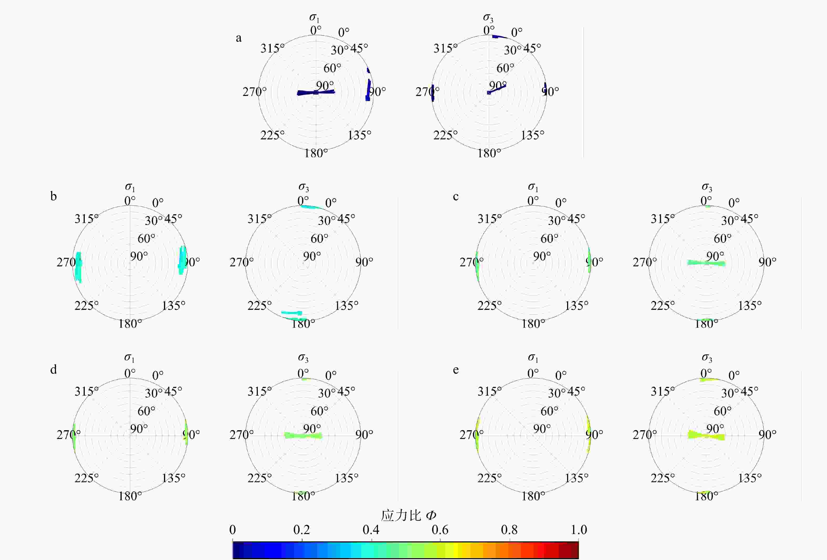
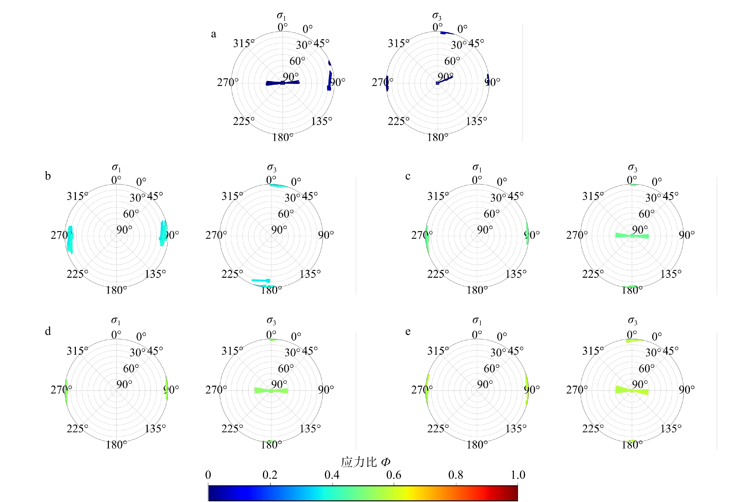
图 10 经过图层分离和帕累托分布优化后的应力反演结果可视化图像
a—应力比位于[0,0.05)区间的分离图像;b—应力比位于[0.35,0.40)区间的分离图像;c—应力比位于[0.45,0.50)区间的分离图像;d—应力比位于[0.50,0.55)区间的分离图像;e—应力比位于[0.55,0.60)区间的分离图像;
Figure 10. Visualization of the stress inversion results after layer separation and Pareto distribution optimization
(a) Separated image for stress ratios within the [0, 0.05) interval; (b) Separated image for stress ratios within the [0.35, 0.4) interval; (c) Separated image for stress ratios within the [0.45, 0.5) interval; (d) Separated image for stress ratios within the [0.5, 0.55) interval; (e) Separated image for stress ratios within the [0.55, 0.6) interval
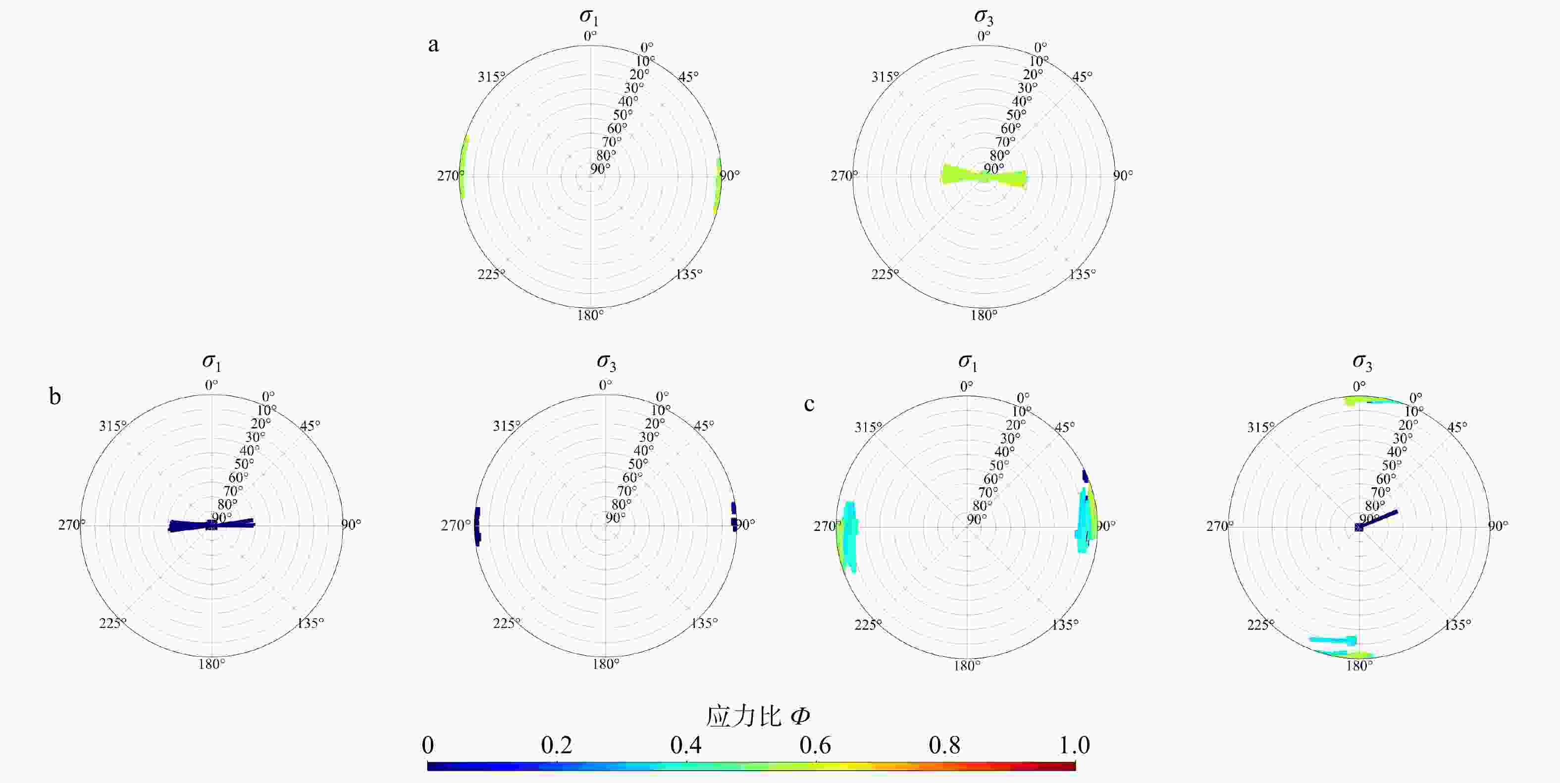
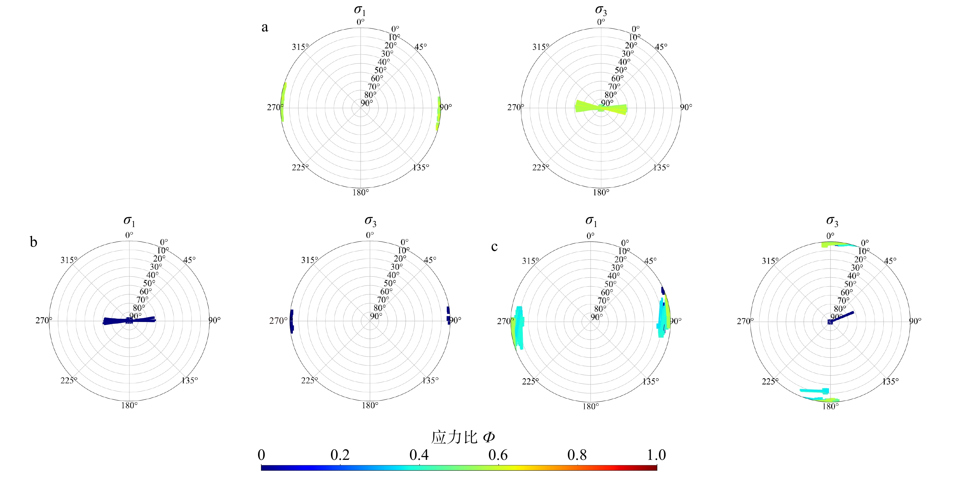
图 11 反演聚类识别结果
a—应力A的聚类识别结果;b—应力B的聚类识别结果;c—应力C的聚类识别结果
Figure 11. Clustering identification results of inversion
(a) Corresponds to the clustering identification result of stress A; (b) Corresponds to the clustering identification result of stress B; (c) Corresponds to the clustering identification result of stress C
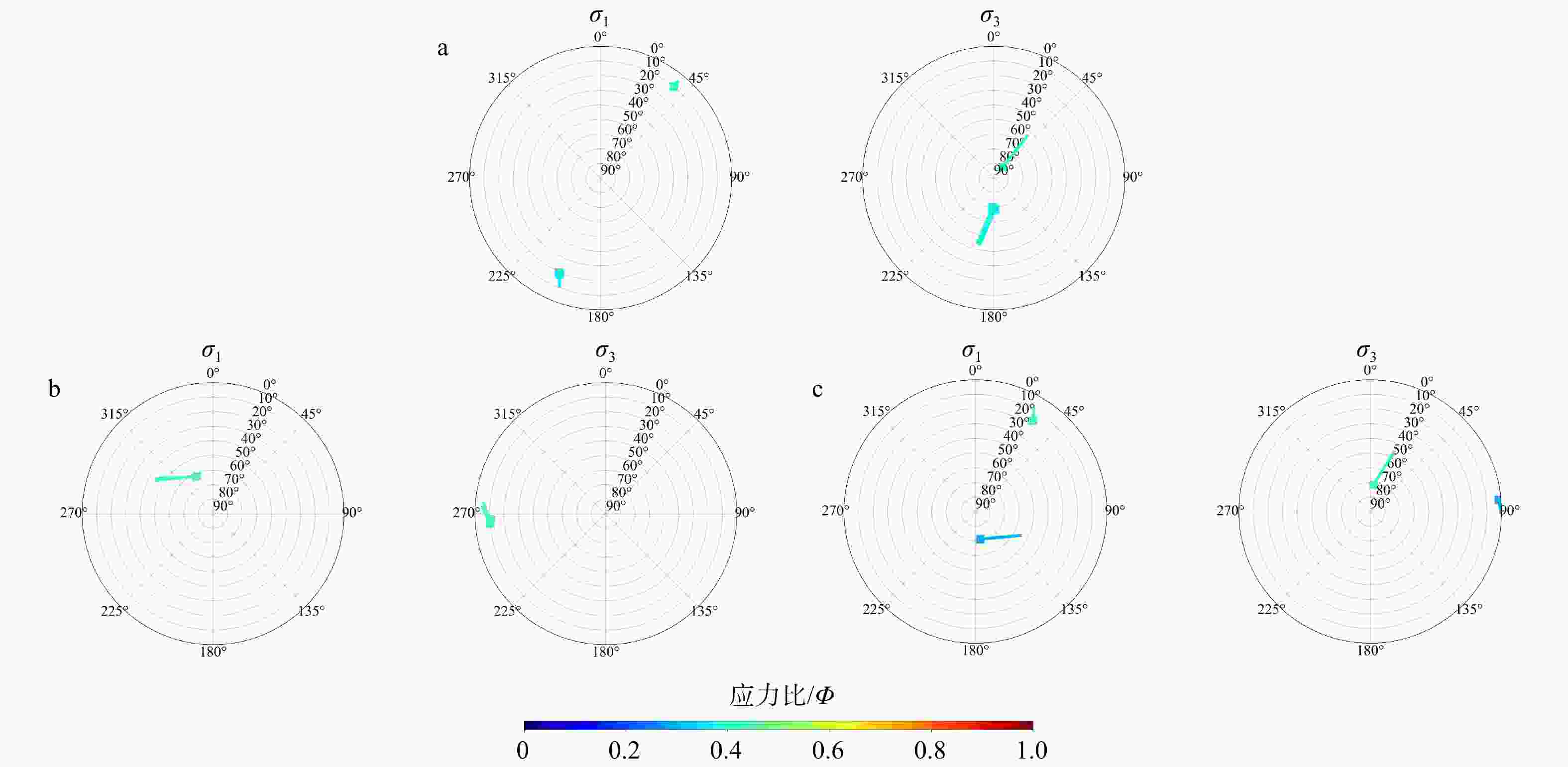
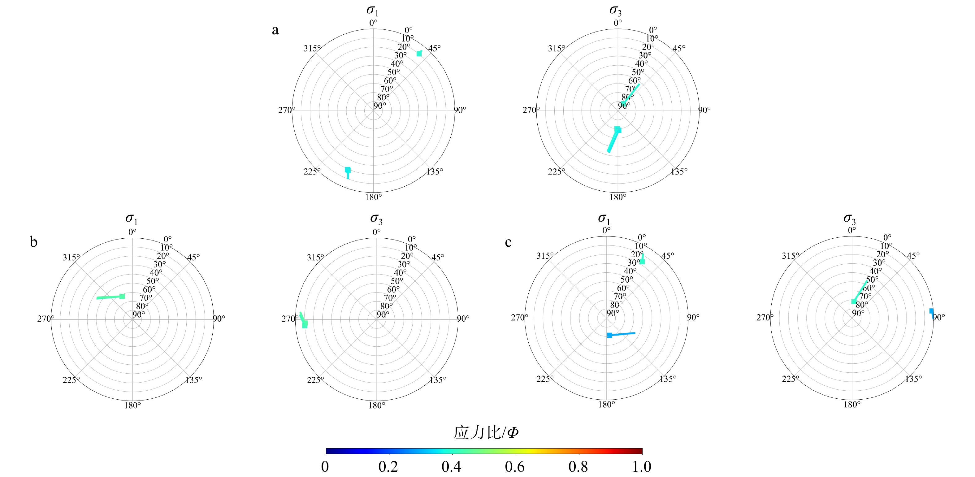
图 12 基于全随机应力加载高斯噪声模型的断层反演结果
a—反演结果1(Ф:0.35~0.4); b—反演结果2(Ф:0.4~0.45);c—反演所用随机应力图像
Figure 12. Faults inversion results based on a Gaussian noise model with fully random stress loading
(a) Inversion result 1 (Ф:0.35–0.4); (b) Inversion result 2 (Ф:0.4–0.45); (c) The random stress used in the inversion
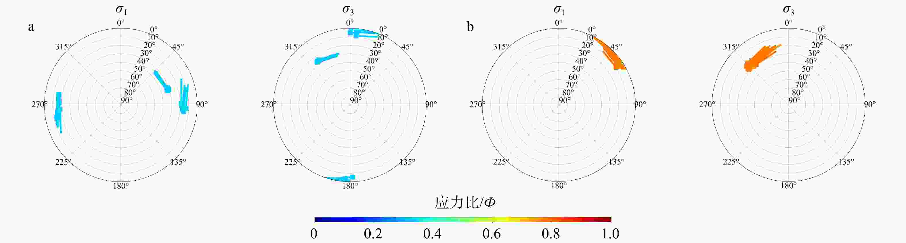
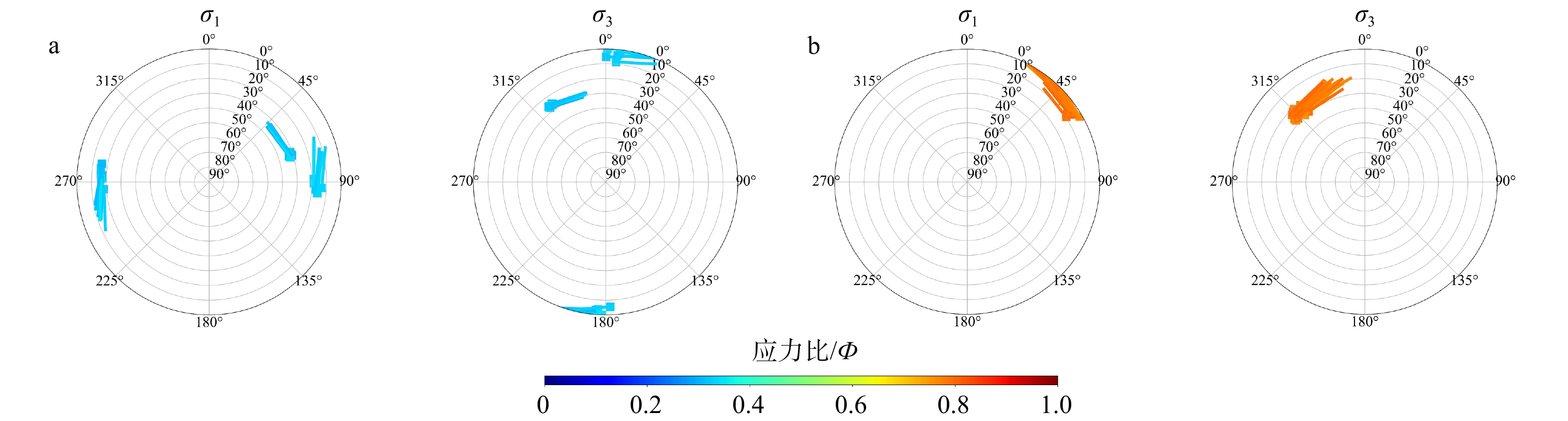
图 13 渤海某区块应力反演后聚类识别结果
a—聚类识别结果1;b—聚类识别结果2
Figure 13. Results of the cluster identification after stress inversion for the study area in the Bohai Sea
(a) Cluster identification result 1; (b) Cluster identification result 2
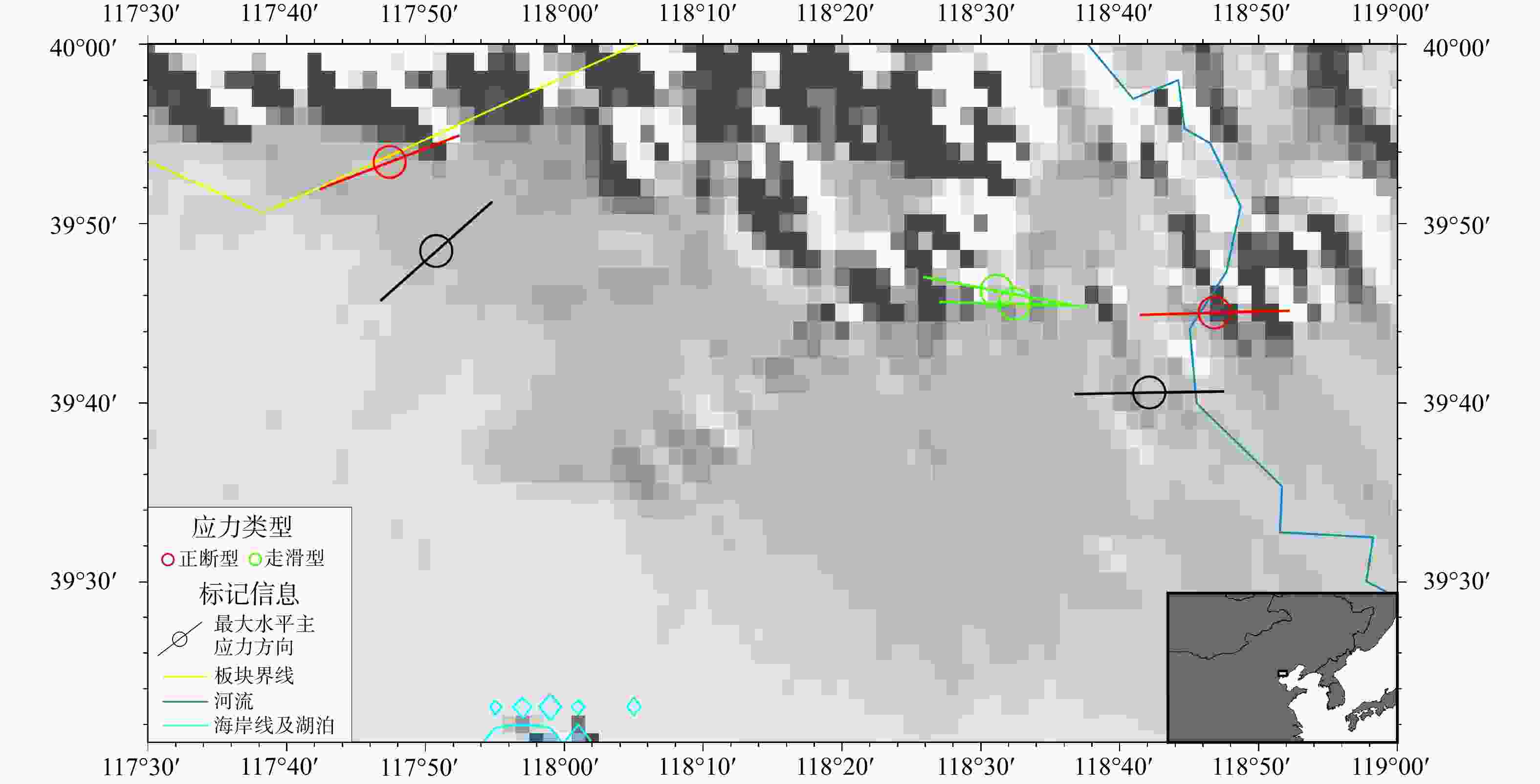
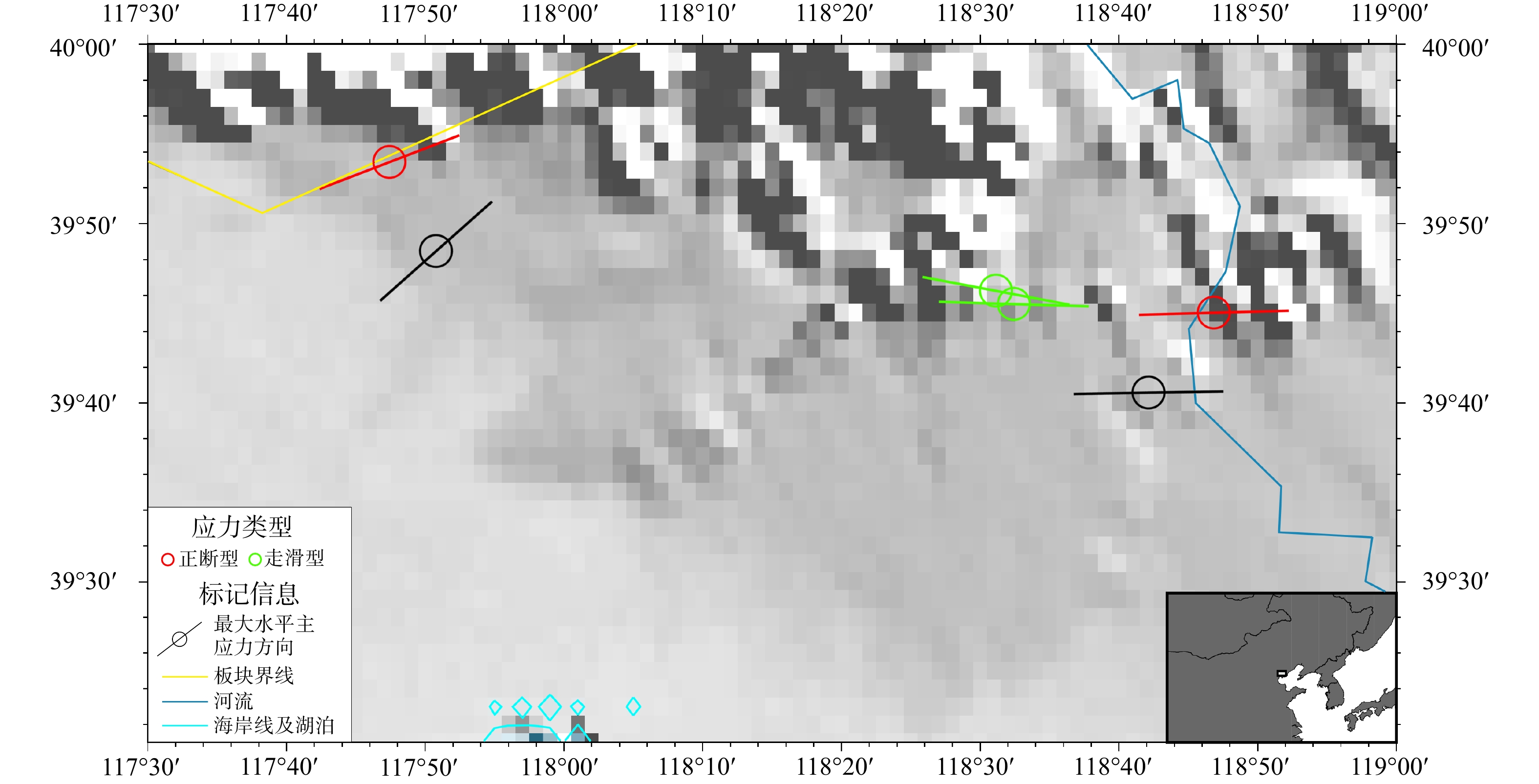
图 14 渤海某区块世界应力地图数据与反演识别最大水平主应力方向结果在地图上的标定
红色和绿色图标为WSM中的数据,黑色图标为反演结果,右下角小图为图中地点在渤海中的位置示意
Figure 14. Calibration of world stress map (WSM) data for the study area in the Bohai Sea and the inversion identification of the maximum horizontal principle stress direction (The red and green icons represent data from the WSM, while the black icons denote the inversion results. The inset in the lower right corner shows the location of the study area within the Bohai Sea.)
表 1 应力参数
Table 1. Stress parameters
序号 α/(°) β/(°) γ/(°) Φ 应力类型 归一化σ A 0 0 0 1/2 逆断型 $ \left[\begin{matrix}\dfrac{\sqrt{6}}{2} & & \\ & 0 & \\ & & -\dfrac{\sqrt{6}}{2}\\ \end{matrix}\right] $ B 0 π/2 0 0 正断型 $ \left[\begin{matrix}\sqrt{2} & & \\ & -\dfrac{\sqrt{2}}{2} & \\ & & -\dfrac{\sqrt{2}}{2}\\ \end{matrix}\right] $ C π/2 π/2 π/2 1/2 走滑型 $ \left[\begin{matrix}\dfrac{\sqrt{6}}{2} & & \\ & 0 & \\ & & -\dfrac{\sqrt{6}}{2}\\ \end{matrix}\right] $  下载: 导出CSV
表 2 随机生成断层参数
Table 2. Randomly generated fault parameters
断层序号 走向θ/(°) 倾向δ/(°) 滑移角λ/(°) 应力类型 断层序号 走向θ/(°) 倾向δ/(°) 滑移角λ/(°) 应力类型 1 347.69 5.51 83.38 A 16 347.34 86.92 −93.65 B 2 31.14 5.39 100.18 A 17 153.27 7.18 −90.11 B 3 118.10 27.93 69.46 A 18 86.82 50.29 −87.59 B 4 305.99 25.48 72.65 A 19 285.11 59.46 −92.17 B 5 321.31 87.83 6.94 A 20 231.99 83.31 −85.17 B 6 158.38 73.96 53.78 A 21 26.96 12.39 146.46 C 7 150.74 69.82 58.47 A 22 37.33 64.76 172.76 C 8 246.45 46.24 115.37 A 23 234.10 58.84 −167.74 C 9 135.36 81.93 27.80 A 24 283.94 15.10 −63.91 C 10 324.52 25.57 71.31 A 25 354.96 27.86 81.27 C 11 103.29 12.48 −88.22 B 26 138.11 1.59 9.92 C 12 69.22 7.76 −94.96 B 27 131.36 28.44 −6.69 C 13 309.09 89.72 −90.06 B 28 152.39 89.83 2.12 C 14 88.74 35.95 −86.05 B 29 16.61 59.23 143.69 C 15 258.40 69.40 −94.10 B 30 320.58 82.14 0.74 C
下载: 导出CSV
表 3 计算硬件与软件环境
Table 3. Computing hardware and software environment
参数名称 配置参数 参数名称 配置参数 计算机型号 IdeaCenter GeekPro – 17IRB 编程语言 Python 3.11.5 CPU Intel Core i7-13700F (16核心,24线程,最高睿频 5.2 GHz) 关键依赖库 NumPy 1.24.3; SciPy 1.11.1; Pandas 2.0.3 RAM 32 GB * 2 3200 MT/s 并行计算库 Joblib 1.2.0 硬盘 SSD 8000 MB/s 1024 GB 集成开发环境 Spyder 5.4.3 操作系统 Windows 11 家庭中文版 版本号 22H2 运算方式 主测试为单进程串行运算;并行测试使用Joblib
下载: 导出CSV
表 4 量子群反演方法与网格搜索法对比
Table 4. Comparison between the QPSO inversion method and the grid search method
比对参数 量子群反演法 网格搜索法 T 831 s 22720 s NN 32 33 反演得到单个结果的平均计算时间t 2.06 s 56.52 s
下载: 导出CSV
表 5 改进量子群反演法与原始量子群反演法对比
Table 5. Comparison between the improved QPSO inversion method and the original QPSO inversion method
比对参数 改进量子群反演法 原始量子群反演法 T 831 s 364 s NN 32 372 反演得到单个结果的平均计算时间t 2.06 s 5.78 s
下载: 导出CSV
表 6 Ⅰ、Ⅱ、Ⅲ聚类信息与模拟断层所用应力张量之间的差值及误差百分比
Table 6. The differences and percentage errors between the clustering information of Ⅰ, Ⅱ, and Ⅲ, and the stress tensor used for simulating the faults
应力参数 聚类Ⅰ 应力A 差值 误差百分比 聚类Ⅱ 应力B 差值 误差百分比 聚类Ⅲ 应力C 差值 误差百分比 σ1轴平均走向夹角 94.320° 90° 4.320° 2.400% 71.868° 90° 18.132° 10.073% 90.436° 90° 0.436° 0.242% σ3轴平均走向夹角 5.702° 0° 5.702° 3.168% 88.547° 90° 1.453° 0.807% 2.205° 0° 2.205° 1.225% σ1轴平均倾角 0.026° 0° 0.026° 0.029% 89.857° 90° 0.143° 0.159% 3.993° 0° 3.993° 4.437% σ3轴平均倾角 89.950° 90° 0.050° 0.056% 0.117° 0° 0.117° 0.13% 4.422° 0° 4.422° 4.913% 平均应力比 0.530 0.5 0.030 3.000% 0.002 0 0.002 0.200% 0.430 0.5 0.070 7.000%
下载: 导出CSV
表 7 随机生成的不规则应力张量
Table 7. Randomly generated irregular stress tensors
序号 α/(°) β/(°) γ/(°) Φ D 354.89 88.40 19.08 0.29 E 276.63 18.37 24.52 0.41
下载: 导出CSV
表 8 加载高斯噪声后的随机断层参数
Table 8. Randomly generated fault parameters after loading Gaussian noise
断层序号 走向θ/(°) 倾向δ/(°) 滑移角λ/(°) 应力类型 断层序号 走向/(°) 倾向δ/(°) 滑移角λ/(°) 应力类型 1 131.70 63.11 −117.03 D 11 240.52 54.82 38.69 E 2 325.75 7.09 −133.07 D 12 31.57 23.66 90.67 E 3 356.00 80.90 −124.48 D 13 159.55 28.16 135.69 E 4 195.11 33.03 −88.80 D 14 8.74 52.91 133.03 E 5 119.38 23.07 −96.16 D 15 263.04 44.55 58.20 E 6 348.25 45.89 −92.83 D 16 182.33 88.73 163.34 E 7 295.56 28.08 −90.57 D 17 338.31 30.37 105.37 E 8 218.53 64.17 −70.16 D 18 189.12 69.51 128.52 E 9 102.98 74.00 −85.65 D 19 136.67 11.87 144.57 E 10 348.73 50.93 −103.99 D 20 135.18 2.87 −178.70 E
下载: 导出CSV
表 9 渤海某区块震源机制信息
Table 9. Focal mechanism information of a certain area in the Bohai Sea
震源查询编号 平面1走向/(°) 平面1倾角/(°) 平面1滑移角/(°) 平面2走向/(°) 平面2倾角/(°) 平面2滑移角/(°) 纬度/(°) 经度/(°) 深度/km 072776A 229 43 −163 126 79 −49 39.52 118.03 15 072876A 72 44 −110 279 49 −71 39.75 118.78 15 111576A 318 56 −9 53 83 −145 39.45 117.71 15 051277B 332 52 8 227 83 142 39.56 118 22 112677C 250 45 −90 70 45 −90 39.89 117.79 15 201205280222A 227 80 172 318 83 10 39.76 118.54 23.5 202007112238A 303 65 −175 33 90 −9 39.77 118.52 23 202212040520A 249 76 −133 145 45 −20 39.88 118.87 10 202104161606A 30 90 −170 300 80 0 39.75 118.71 9 202007120638A 135 78 −42 236 49 −164 39.78 118.44 10
下载: 导出CSV
表 10 渤海某区块应力反演结果聚类的平均参数
Table 10. The average parameters of the clustering results of stress inversion for the study area in the Bohai Sea
聚类结果 σ1轴平均走向夹角 σ1轴平均倾角 σ3轴平均走向夹角 σ3轴平均倾角 平均应力比 聚类识别结果1 86.230° 21.472° −8.829° 9.961° 0.327 聚类识别结果2 49.514° 3.167° 138.191° 23.699° 0.777
下载: 导出CSV
-
[1] AKI K, Richards P G. Quantitative seismology[M]. 2002. [2] AN J L, LIU X N, HE M, et al., 2022. Survey of quantum swarm intelligence optimization algorithm[J]. Computer Engineering and Applications, 58(7): 31-42. (in Chinese with English abstract) [3] ANDERSON E M, 1905. The dynamics of faulting[J]. Transactions of the Edinburgh Geological Society, 8(3): 387-402. doi: 10.1144/transed.8.3.387 [4] ANDERSON E M, 1951. The dynamics of faulting and dyke formation with applications to Britain[M]. Edinburgh: Oliver & Boyd. [5] ANGELIER J, 1979. Determination of the mean principal directions of stresses for a given fault population[J]. Tectonophysics, 56(3-4): T17-T26. doi: 10.1016/0040-1951(79)90081-7 [6] ANGELIER J, 1984. Tectonic analysis of fault slip data sets[J]. Journal of Geophysical Research: Solid Earth, 89(B7): 5835-5848. doi: 10.1029/JB089iB07p05835 [7] ANGELIER J, 1990. Inversion of field data in fault tectonics to obtain the regional stress: III. A new rapid direct inversion method by analytical means[J]. Geophysical Journal International, 103(2): 363-376. doi: 10.1111/j.1365-246X.1990.tb01777.x [8] BOTT M H P, 1959. The mechanics of oblique slip faulting[J]. Geological Magazine, 96(2): 109-117. doi: 10.1017/S0016756800059987 [9] DIDAY E, 1971. Une nouvelle méthode en classification automatique et reconnaissance des formes la méthode des nuées dynamiques[J]. Revue de Statistique Appliquée, 19(2): 19-33. [10] DUAN H B, 2005. Ant colony algorithms: theory and applications[M]. Beijing: Science Press. (in Chinese with English abstract) [11] DZIEWONSKI A M, CHOU T A, WOODHOUSE J H, 1981. Determination of earthquake source parameters from waveform data for studies of global and regional seismicity[J]. Journal of Geophysical Research: Solid Earth, 86(B4): 2825-2852. doi: 10.1029/JB086iB04p02825 [12] EBERHART R, KENNEDY J, 1995. A new optimizer using particle swarm theory[C]//MHS'95. Proceedings of the sixth international symposium on micro machine and human science. Nagoya: IEEE: 39-43. [13] EKSTRÖM G, NETTLES M, DZIEWOŃSKI A M, 2012. The global CMT project 2004-2010: centroid-moment tensors for 13, 017 earthquakes[J]. Physics of the Earth and Planetary Interiors, 200-201: 1-9. [14] GUAN L, JIANG G M, 2023. High-precision Earthquake Locations and Deep Fault Characteristics Beneath Xianyou Area, Fujian Province[J]. Geoscience, 37(01): 40-47. (in Chinese with English abstract) [15] HE Z Y, REN X H, LIU Y, 2010. Back analysis of initial ground stress based on FLAC3D and particle swarm optimization[J]. Water Resources and Power, 28(8): 46-48. (in Chinese with English abstract) [16] HEIDBACH O, RAJABI M, DI GIACOMO D, et al. , 2025. World Stress Map 2025. GFZ Data Services, doi: 10.5880/WSM.2025.002 [17] HUANG Q, 1988. Computer-based method to separate heterogeneous sets of fault-slip data into sub-sets[J]. Journal of Structural Geology, 10(3): 297-299. doi: 10.1016/0191-8141(88)90062-4 [18] LI X, XIE X B, YANG C X, et al. , 2015. Inversion analysis of initial stress field based on modified particle swarm optimization[J]. Mining and Metallurgical Engineering, 35(1): 23-26, 30. (in Chinese with English abstract) [19] LI X W, ZHANG G W, XIE Z J, et al., 2022. Characteristics of the focal mechanism solution and the present stress field in the Bohai Sea Region[J]. Earthquake Research in China, 38(4): 708-720. (in Chinese with English abstract) [20] LIU J J, LU Y S, WANG Q Z, et al., 2012. Application of particle swarm optimization with quantum behavior(QPSO) to logging inversion[J]. Chinese Journal of Engineering Geophysics, 9(2): 151-154. (in Chinese with English abstract) [21] NEMCOK M, RICHARD J L, 1995. A stress inversion procedure for polyphase fault/slip data sets[J]. Journal of Structural Geology, 17(10): 1445-1453. doi: 10.1016/0191-8141(95)00040-K [22] ORIFE T, LISLE R J, 2003. Numerical processing of palaeostress results[J]. Journal of Structural Geology, 25(6): 949-957. doi: 10.1016/S0191-8141(02)00120-7 [23] OTSUBO M, YAMAJI A, 2006. Improved resolution of the multiple inverse method by eliminating erroneous solutions[J]. Computers & Geosciences, 32(8): 1221-1227. [24] OTSUBO M, YAMAJI A, KUBO A, 2008. Determination of stresses from heterogeneous focal mechanism data: an adaptation of the multiple inverse method[J]. Tectonophysics, 457(3-4): 150-160. doi: 10.1016/j.tecto.2008.06.012 [25] SATO K, YAMAJI A, 2006. Uniform distribution of points on a hypersphere for improving the resolution of stress tensor inversion[J]. Journal of Structural Geology, 28(6): 972-979. doi: 10.1016/j.jsg.2006.03.007 [26] SIMPSON R W, 1997. Quantifying Anderson's fault types[J]. Journal of Geophysical Research: Solid Earth, 102(B8): 17909-17919. doi: 10.1029/97JB01274 [27] SUN J, 2009. Particle swarm optimization with particles having quantum[D]. Wuxi: Jiangnan University. (in Chinese with English abstract) [28] WALLACE R E, 1951. Geometry of shearing stress and relation to faulting[J]. The Journal of Geology, 59(2): 118-130. doi: 10.1086/625831 [29] WANG P Q, LIU X Y, LI Q C, et al., 2025. Research on multi-wave joint elastic modulus inversion based on improved quantum particle swarm optimization[J]. Petroleum Science, 22(2): 670-683. doi: 10.1016/j.petsci.2024.10.006 [30] WANG R Y, WAN Y K, GUAN Z X, et al., 2025. Static stress triggering of morocco M6.9 earthquake on 9 September 2023[J]. Journal of Geomechanics, 31(2): 223-234. (in Chinese with English abstract) [31] YAMAJI A, 2000. The multiple inverse method: a new technique to separate stresses from heterogeneous fault-slip data[J]. Journal of Structural Geology, 22(4): 441-452. doi: 10.1016/S0191-8141(99)00163-7 [32] YAMAJI A, SATO K, 2006. Distances for the solutions of stress tensor inversion in relation to misfit angles that accompany the solutions[J]. Geophysical Journal International, 167(2): 933-942. doi: 10.1111/j.1365-246X.2006.03188.x [33] YAMAJI A, SATO K, 2012. A spherical code and stress tensor inversion[J]. Computers & Geosciences, 38(1): 164-167. [34] YANG G T, 2004. Introduction to elasticity and plasticity[M]. Beijing: Tsinghua University Press. (in Chinese with English abstract) [35] YANG Z G, XU T R, LIANG J H, 2024. Towards fast focal mechanism inversion of shallow crustal earthquakes in the Chinese mainland[J]. Earthquake Research Advances, 4(2): 100273. doi: 10.1016/j.eqrea.2023.100273 [36] ZHANG G Y, WU Y G, GU W, 2013. Quantum-behaved particle swarm optimization algorithm based on elitist learning[J]. Control and Decision, 28(9): 1341-1348. (in Chinese with English abstract) [37] ZHAO Y F, SHI W, ZHANG Y, 2023. Study on the reconstruction of the paleo-tectonic stress field and its evolution in the Jinchuan mining district, Gansu Province, China[J]. Journal of Geomechanics, 29(6): 770-785. (in Chinese with English abstract) [38] ZOBACK M D, 2010. Reservoir geomechanics[M]. Cambridge: Cambridge University Press. [39] 安家乐, 刘晓楠, 何明, 等, 2022. 量子群智能优化算法综述[J]. 计算机工程与应用, 58(7): 31-42. doi: 10.3778/j.issn.1002-8331.2110-0141 [40] 段海滨, 2005. 蚁群算法原理及其应用[M]. 北京: 科学出版社. [41] 关露凝, 江国明, 2023. 福建仙游地区高精度地震震源定位及深部断裂特征[J]. 现代地质, 37(1): 40-47 [42] 何竹叶, 任旭华, 刘燕, 2010. 基于FLAC3D和粒子群优化算法的初始地应力场反演[J]. 水电能源科学, 28(8): 46-48. doi: 10.3969/j.issn.1000-7709.2010.08.015 [43] 李欣, 谢学斌, 杨承祥, 等, 2015. 基于改进粒子群优化算法的地应力场反演[J]. 矿冶工程, 35(1): 23-26, 30. doi: 10.3969/j.issn.0253-6099.2015.01.007 [44] 李欣蔚, 张广伟, 谢卓娟, 等, 2022. 渤海海域地震震源机制解与现今应力场特征[J]. 中国地震, 38(4): 708-20. doi: 10.3969/j.issn.1001-4683.2022.04.009 [45] 刘建军, 卢以水, 王全洲, 等, 2012. 量子粒子群算法在测井反演解释中的应用[J]. 工程地球物理学报, 9(2): 151-154. doi: 10.3969/j.issn.1672-7940.2012.02.005 [46] 孙俊, 2009. 量子行为粒子群优化算法研究[D]. 无锡: 江南大学. [47] 王润妍, 万永魁, 关兆萱, 等, 2025. 2023年9月9日摩洛哥M6.9地震静态应力触发研究[J]. 地质力学学报, 31(2): 223-234. doi: 10.12090/j.issn.1006-6616.2024039 [48] 杨桂通, 2004. 弹塑性力学引论[M]. 北京: 清华大学出版社. [49] 章国勇, 伍永刚, 顾巍, 2013. 基于精英学习的量子行为粒子群算法[J]. 控制与决策, 28(9): 1341-1348. doi: 10.13195/j.kzyjc.2013.09.015 [50] 赵远方, 施炜, 张宇, 2023. 甘肃金川矿区古构造应力场恢复及演化研究[J]. 地质力学学报, 29(6): 770-785. doi: 10.12090/j.issn.1006-6616.2023161 -

 下载:
下载:


计量
- 文章访问数: 354
- HTML全文浏览量: 110
- PDF下载量: 114
- 被引次数: 0
